Introduction

The Tond Tenga Project in Burkina Faso was the first Verified Carbon Standard (VCS) project. As part of their biomass stocking index methodology, they use the Normalized Difference Fraction Index (NDFI), calculated from Landsat 8 and 9 Operational Land Imager (OLI) scenes. This catch my interest and motivated me to revisit the method. In this blog, I’ll write down my notes and key takeaways, both for my own reference and for others who want to understand the core ideas behind the NDFI.

At first glance, the name sounds similar to other well-known remote sensing indices like NDVI or NDWI. But unlike those indices, NDFI isn’t a simple equation applied to standard satellite bands. In fact, I think NDFI adaptation in remote sensing should be seen more as a general concept or approach in feature engineering, rather than a fixed index. Let’s unpack that in more detail.

A Quick Look at Spectral Mixture Analysis (SMA)

NDFI was originally developed to map forest canopy damage caused by selective logging and fires in the Amazon, introduced by Souza et al. (2005). It’s based on a method called spectral mixture analysis (SMA), or spectral unmixing. It is something I’ve write multiple time in this blog before. But for completeness, let’s go over a quick refresher.

SMA starts from a classic remote sensing problem: a single pixel often contains multiple objects. For example, take the pixel shown in the image below:

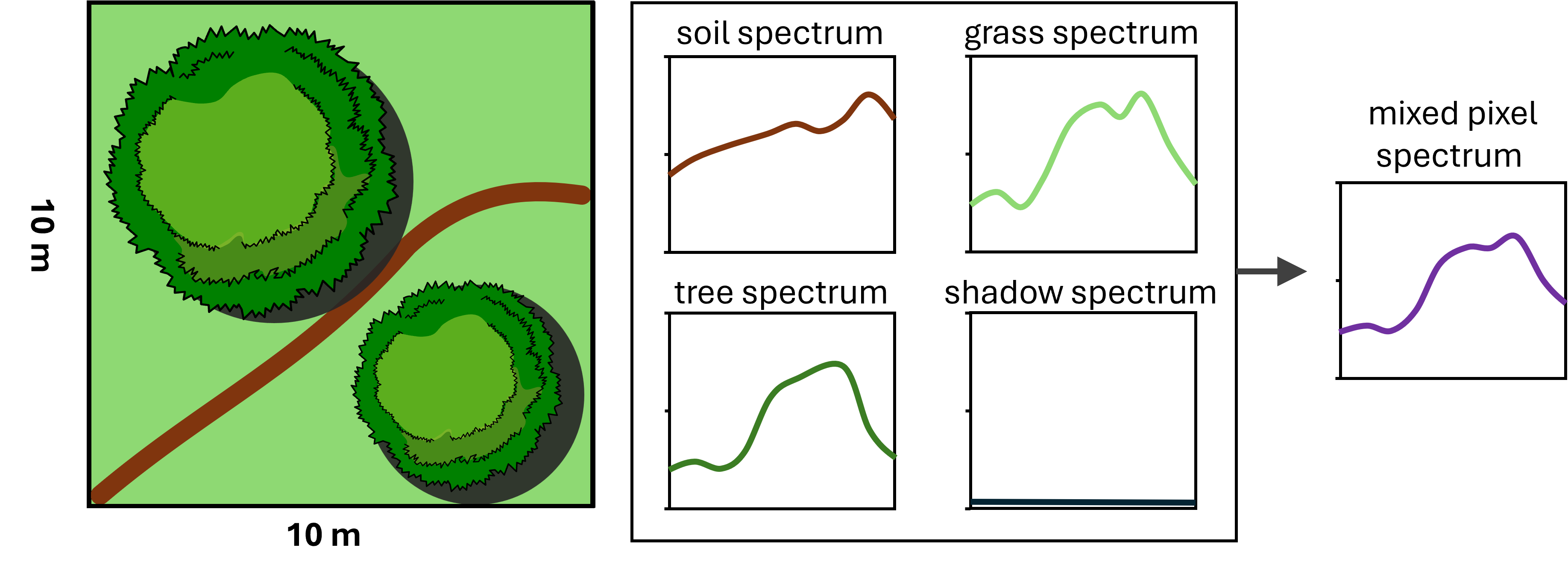
Within that one 10 x 10 m pixel, we have two tree crowns, some grassy ground, and part of a dirt road. In SMA, these individual components are called endmembers. From spectroscopy, we know that different materials reflect and absorb light in different ways, this behavior across wavelengths is what we call a spectral signature.

Trees, grass, and soil each have their own characteristic spectral signatures. In multispectral or hyperspectral images, these differences let us distinguish one endmember from another. But when several endmember are mixed within a single pixel, the resulting spectral signal is a mixed spectrum, and that makes it harder to classify the pixel using a simple “match-the-spectrum” approach.

SMA becomes useful for two main reasons. First, because a mixed pixel hides the original spectral signature of each object, it becomes hard to classify each pixel directly using traditional approaches. SMA helps us make sense of that mix. Second, sometimes we want to get more detailed information than what the resolution of the image allows. For example, we might want to estimate the tree canopy cover inside a single pixel, even if that pixel covers 10 or 30 meters on the ground. SMA lets us break down that pixel and estimate the proportion of each endmembers inside it.

SMA typically assumes a linear mixing model, where each endmember’s spectral signature is multiplied by its area fraction, and then summed. In matrix notation we can write it as:

Where \(\mathbf{y}\) is the mixed spectra that the sensor capture, \(\mathbf{E}\) is the endmember spectra matrix where each vertical component represent a single endmemebr spectra, and \(\mathbf{a}\) is the area fraction vector which is summed to one.

In most SMA workflows, we assume that the endmembers spectra \(\mathbf{E}\) is known. We won’t go into how to extract the endmembers here, but common approaches include using spectral libraries, manually selecting the purest pixels, or applying automated methods like NFINDR, which I’ve explained in more detail here.

The main goal is to solve for the vector \(\mathbf{a}\), which gives us the area fraction of each endmembers inside the pixel. This is usually done by solving a constrained optimization problem (non-negative, sum-to-one constraints). You can refer to the equation I used in my earlier post here.

Now, is the linear mixing assumption reasonable? This assumption holds true if we assume a completely flat and smooth surface as ilustrated in the image below.

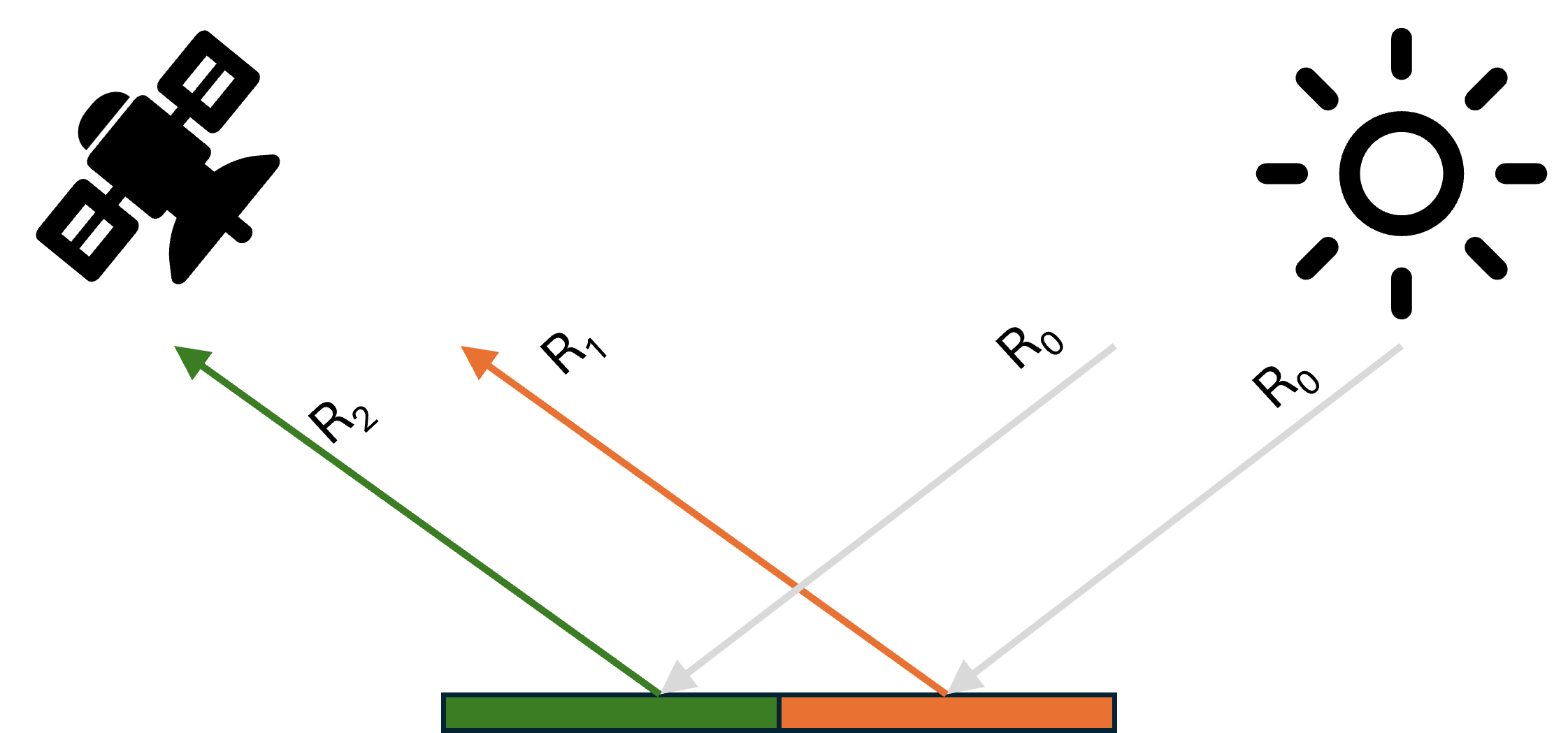
In this scenario, each light ray from the sun (\(\mathbf{R}_0\)) interacts with only one object before reflecting into the sensor. In this case both \(\mathbf{R}_1\) and \(\mathbf{R}_2\) are pure reflectance (endmember’s spectral signature) of object 1 and object 2, respectively. What the sensor receives is simply a linear combination of these reflectances weighted by their respective area fractions.

However, real-world surfaces are obviously more complex. For example, consider the next image, which better reflects a realistic, vegetated surface:

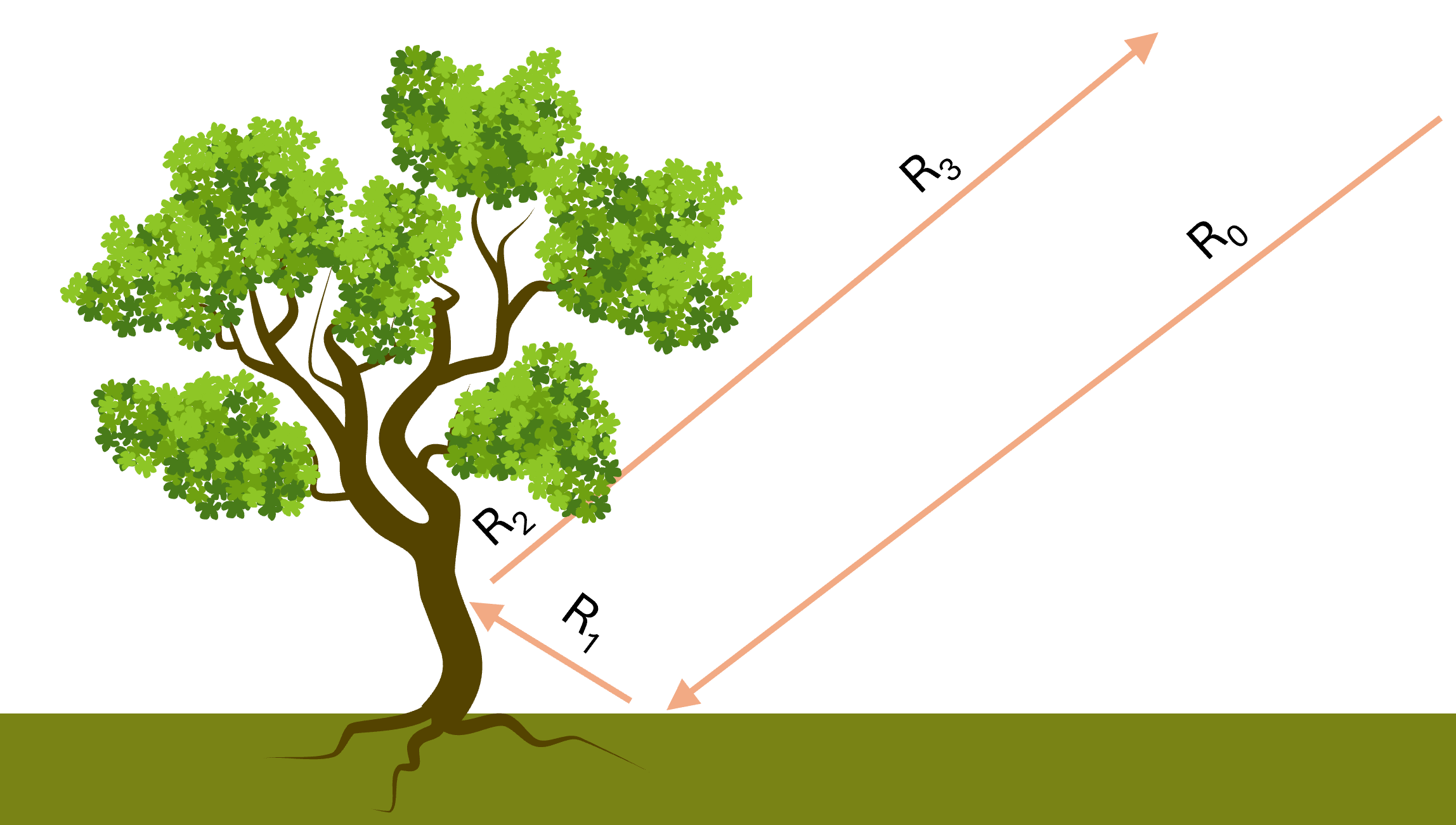
Due to the complex condition of the real surface, light doesn’t just bounce off one object. It often reflects multiple times between different objects before reaching the sensor. For instance, in the image above, \(\mathbf{R}_1\) is the normal reflectance from the ground, this will be equal to the ground spectral signature. Then we have \(\mathbf{R}_2\), which is the reflectance from the tree trunk. But here, the light hitting the trunk isn’t direct sunlight anymore, it is already been reflected off the ground. So if we have a reference endmember spectrum for tree bark, it will not be equal to \(\mathbf{R}_2\), because endmember spectrum was measured assuming direct sunlight as the source. Finally, \(\mathbf{R}_3\) becomes even more complex, as it involves multiple reflections of light that already reflected multiple times. These multi-bounce interactions are why the signal the sensor receives doesn’t follow a simple linear mixture of the endmembers spectra. The assumption breaks down when multiple scattering effects become significant.

I bring this up because I think it is important to be aware of the limitation of this approach and to acknowledge that there are methods that try to model this more realistically. For example, bilinear mixing models have been shown to perform better in vegetated areas. I also discussed a more physics-based nonlinear model in my earlier research on mineral mixtures.

That said, modeling the precise interaction of light and matter on Earth’s surface is, for most practical purposes, nearly impossible. And once you go down that path, it’s easy to over-engineer the problem and fall into a rabbit hole: adding tons of complexity for only marginal performance gains.

It helps to remember that each time light reflects, it loses intensity. So usually, the strongest contribution to the final signal is from the first object the light hits. For a lot of real-world remote sensing tasks, the linear model gives a good enough approximation. If it doesn’t, then it’s time to explore something more complex.

NDFI

After a long (but necessary) introduction about SMA, now it’s time to talk about NDFI itself.

In the original paper, the authors used Green Vegetation (GV), Non-Photosynthetic Vegetation (NPV), Soil, and Shadow as their endmembers. Since their goal was to detect selectively logged and burned forest, these were the classes they considered useful. The underlying idea is that undisturbed forest has a high proportion of GV, while disturbed forest has more NPV and Soil. So in the original implementation, NDFI grouped all green vegetation into a single GV class.

However, when we apply regular spectral unmixing in forested areas, we run into a common problem: shadows. Forest canopies often cast strong shadows, which can dominate parts of the spectral signal and throw off the GV proportion. To correct for this, the original method normalized the GV fraction by the proportion of non-shadow in the pixel:

After this correction, they calculated the normalized difference between the corrected GV and the combined NPV + Soil fraction using this equation:

This simple adjustment makes a big difference. By correcting GV with shadow and structuring the index around the key land cover fractions, NDFI performs very well for what it was originally designed to do.

However, if we want to use NDFI for a different purpose, for example as a predictor for above-ground biomass (ABG), then a critical adaptation of the index may be useful. Intuitively, I think separating trees from grass or shrubs would be helpful, since they have very different biomass, even though both are green vegetation.

The main concept of NDFI still holds. What changes is the definition of the endmembers and how we combine them in the index. For instance, in a biomass mapping application, we may want to compute the proportion of tree cover relative to all other land cover types (grass, shrub, NPV, soil, etc). That way, NDFI becomes more aligned with the information we care about.

And of course, endmember selection is flexible. Different ecoregions may require different class definitions depending on which surface types are important—or which ones can be safely ignored.

Example: NDFI in Tropical Forest Using Sentinel-2

Let’s use Sentinel-2 imagery to look at a tropical rainforest area in Borneo as an example. Below is the RGB image of the area, along with the NDFI result. The NDFI here is computed using Tree, Grass, Soil, and Shadow as the endmembers. The endmembers spectra were extracted manually from the image.

There are some buildings visible, but I didn’t include them as endmembers since they’re irrelevant for this analysis. I also couldn’t find a convincing candidate for NPV in this area, so I excluded it. Therefore, the NDFI in this example is calculated by comparing the shadow-corrected Tree fraction with the sum of Grass and Soil fractions.

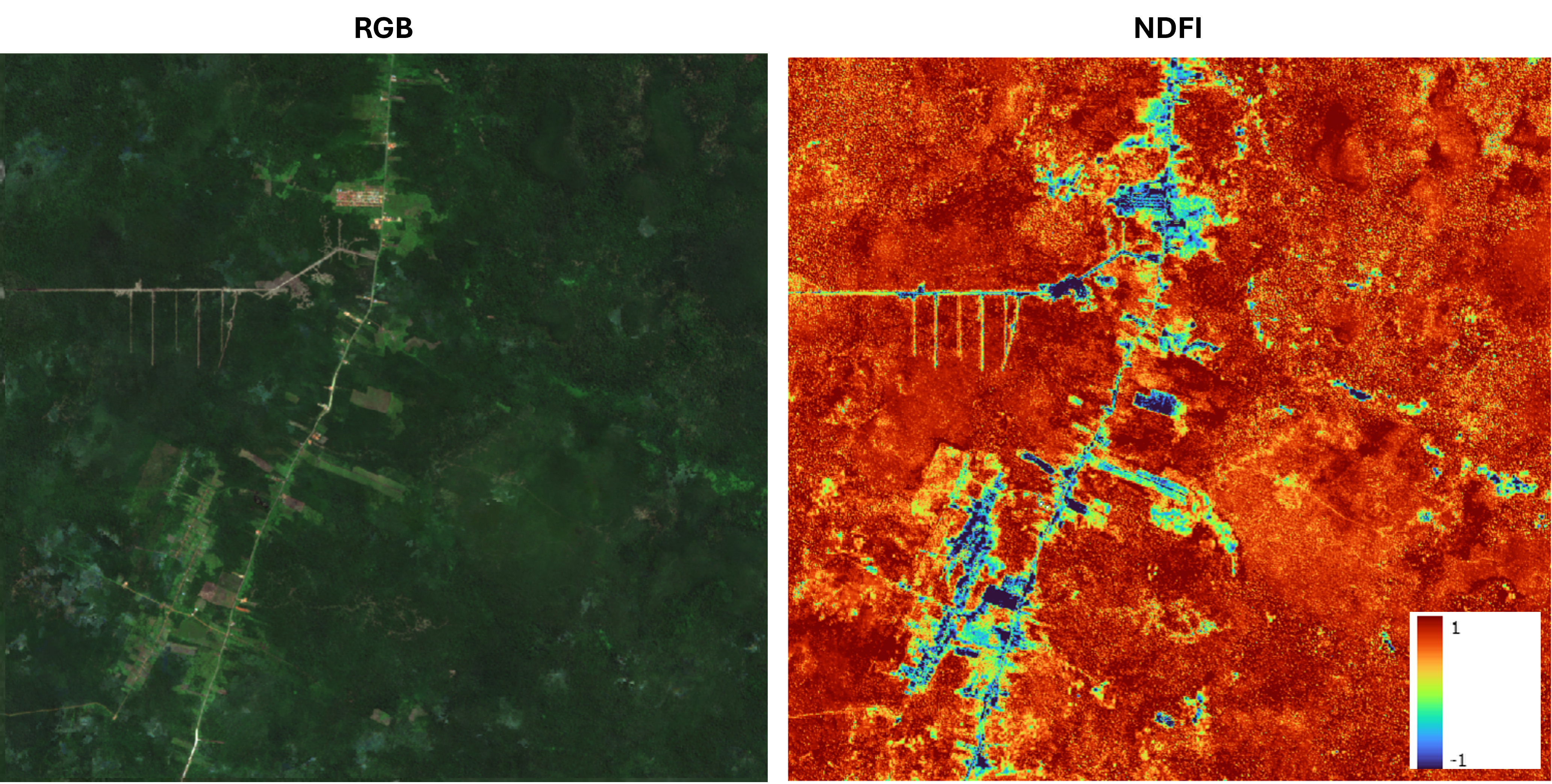
A high NDFI value (shown in red) indicates a higher proportion of tree canopy inside a pixel, which usually suggests denser forest. Areas in yellow or orange still have tree canopy dominance, but are less dense. Regions in green to blue have minimal or no tree cover.

Even visually, we can already see that this image helps distinguish dense forest, which likely has higher AGB, from sparser or degraded forest. In the context of a stocking index, the next step would be to explore the relationship between this NDFI output and AGB modeled from field measurements.

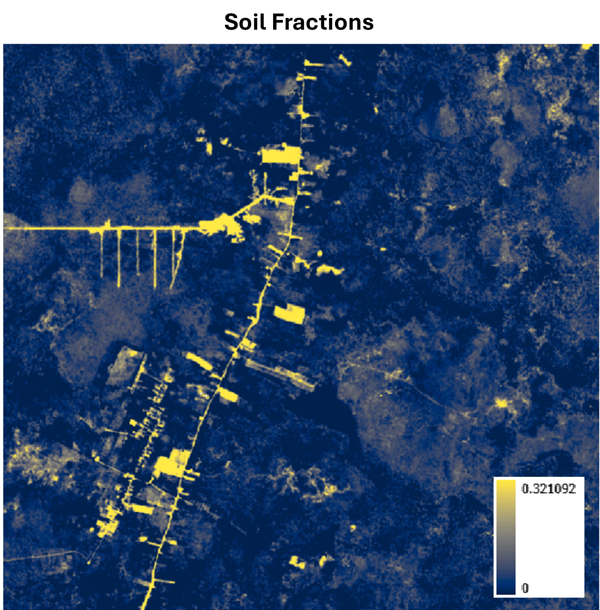
It’s also important to point out that generating NDFI requires us to first compute the fractional abundance of each endmember from the spectral unmixing. This intermediate result can be useful on its own. For instance, the Soil fraction alone is quite effective at highlighting small roads, which can be a valuable input layer for downstream tasks like road detection using deep learning.

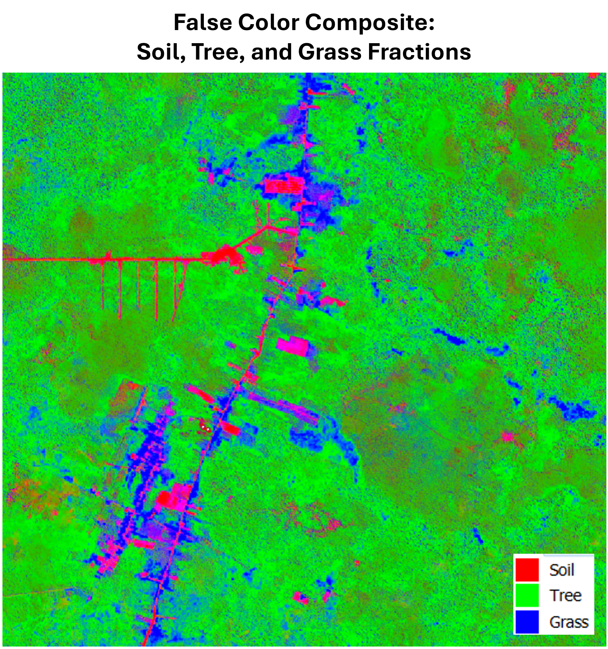
And for standard visualization purposes, it’s also useful to combine the fraction layers into a false color composite to visualize how different land cover types are distributed spatially.

My Takeaway

I was doing a quick research about above-ground biomass when I stumbled back upon this method. While thinking more carefully about it, and while writing this post, I realized a few important general takeaways about doing remote sensing analysis.

First, it’s tempting to just take some well-known equation, apply it to our data, and call it a day. On the other extreme, we might overthink the physics and math behind the problem, end up overengineering the solution, and spend a lot of time, effort, and money, only to gain marginal improvements in the final result.

Ideally, we should aim for something in between. We invest time early on to build a solid understanding of the fundamentals, clarify the real goal of the analysis, and consider the available resources. Then we design a solution that balances practicality, accuracy, and efficiency.

In the end, good remote sensing work is not just about applying the right method, but about applying the right level of thinking about the goal, the problem, the solution, and the constraint.