Different Distance Metrics Example in Spectral Unmixing

In data space, distance is commonly used to measure the similarity between data points. For instance, if points a and b are “close” to each other (i.e., have a small distance), they are considered more similar. This concept is essential in machine learning and data analysis as it can be used to quantifies similarity between datasets.

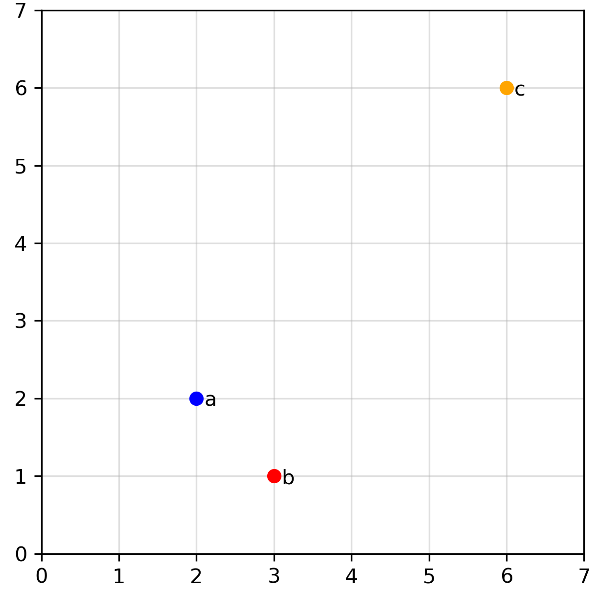
In two dimensions, it’s easy to visualize data points and assess their distances, such as in this example:

Visually, most of us would agree that points a and b appear closer in distance to each other compared to a and c. But is this really the case? To confirm, we need to define what we mean by “distance” and calculate the distance between each point.

In this post, we will examine three different distance metrics and compare their performance in a hypothetical spectral unmixing problem: Euclidean distance, Manhattan distance, and angular distance. I think it is easier to first take a look the visualization of how each metrics measure distance:

I think this ilustration cleary shows the distinction between how the three metrics measure distance, to formalize this, let’s go to each metrics and see its mathematical formulation.

Euclidean Distance

The most common and intuitive distance is Euclidean distance, also often referred to as \(L_2\) distance. Between two points \(a\) and \(b\) in data space, Euclidean distance is simply the straight-line distance between the points, which can be expressed mathematically as:

\[L_2 = \sqrt{\sum_{i=1}^n (a_i - b_i)^2}\]

Manhattan Distance

Another way to measure distance from \(a\) to \(b\) is to follow a path parallel to the axis. For example, in the image below, we first move parallel to the y-axis for 1 units, followed by a parallel path along the x-axis for 1 units, and then sum the total path length. This type of “gridded” path is called Manhattan distance (after the gridded road pattern of Manhattan) or \(L_1\) distance. Mathematically, it can be expressed as:

\[L_1 = \sum_{i=1}^n |a_i - b_i|\]

Angular Distance

For angular distance \((\theta)\), we treat points \(a\) and \(b\) as two vectors originating from the origin \((0,0)\). The angular distance is simply the angle between the two vectors, expressed as:

\[\theta = \arccos \left( \frac{a \cdot b}{\|a\| \|b\|} \right)\]

In machine learning, angular distance is more commonly referred to as cosine similarity (measured as the cosine of the angle). In spectral analysis, this is often called Spectral Angle Mapping (SAM) and is widely used for spectral matching. Mathematically, angular distance is only valid as a metric if we normalize our data to unit vectors. For unit vectors, this measurement gives the same result as Euclidean distance after normalizing the data.

From these definitions of the three distance metrics, lets return to our initial visualization (Image 1): Is point a closer to point b than to point c ? Again, the answer depends on the distance metric. Using Euclidean and Manhattan distances, this statement holds true. However, with angular distance, it is actually false, while a and b have a non-zero angular distance, a and c actually have an angular distance of \(0\). So using this metric, c is closer to a compared to b! I think this simple example already ilustrate how crutial it is to understand the distinction between different distance metrics and in which cases using one is prefered compared to the others.

Example Case: Linear Spectral Unmixing

To illustrate cases in which each distance metric is more appropriate, let’s use linear spectral unmixing as an example. Spectral unmixing is an important analytical technique in remote sensing used to decompose mixed pixel values into their constituent spectral signatures, known as endmembers, and their respective abundances. This process is essential for applications requiring sub-pixel level analysis, such as land cover classification, resource exploration, and environmental monitoring.

An important aspect of spectral unmixing is the choice of distance metrics, which measure the similarity or dissimilarity between observed pixel spectra and modeled spectra. The selection of an appropriate metric significantly impacts the accuracy and performance of unmixing algorithms. Understanding these metrics helps optimize the unmixing process, especially in scenarios with high spectral variability or noise.

Assuming a linear mixture model, a mixed spectrum of several different endmembers is defined as:

\[\mathbf{y} = \mathbf{E} \mathbf{a} + \mathbf{n}\]

where:

• \(\mathbf{y}\) is the observed spectrum,
• \(\mathbf{E}\) is the endmembers matrix,
• \(\mathbf{a}\) is the abundance vector,
• \(\mathbf{n}\) represents noise.

In this equation, \(\mathbf{y}\) is known from observation, and for simplicity, we assume that a matrix of possible endmembers \(\mathbf{E}\) is also known, and noise \(\mathbf{n}\) is negligible.

The goal is to solve for \(\mathbf{a}\) by minimizing the difference between the modeled spectrum \(\mathbf{E} \mathbf{a}\) and the observed spectrum \(\mathbf{y}\), under the conditions that all values of \(\mathbf{a}\) are non-negative and summed-to-one. This may achieved by solving this optimization problem:

\[\min_{\mathbf{a}} \; D(\mathbf{y} - \mathbf{E} \mathbf{a})\]

subject to:

\[\mathbf{a}_i \geq 0 \quad \text{and} \quad \sum_{i=1}^{n} \mathbf{a}_i = 1\]

This is where distance metrics \(D(•)\) come into play. The difference we are trying to minimize can be calculated using different distance metrics. Different distance metrics can lead to different results.

Now, let’s run some tests under various simplified scenarios to see how each distance metric performs.

Test 01: Mixture with Gaussian Noise

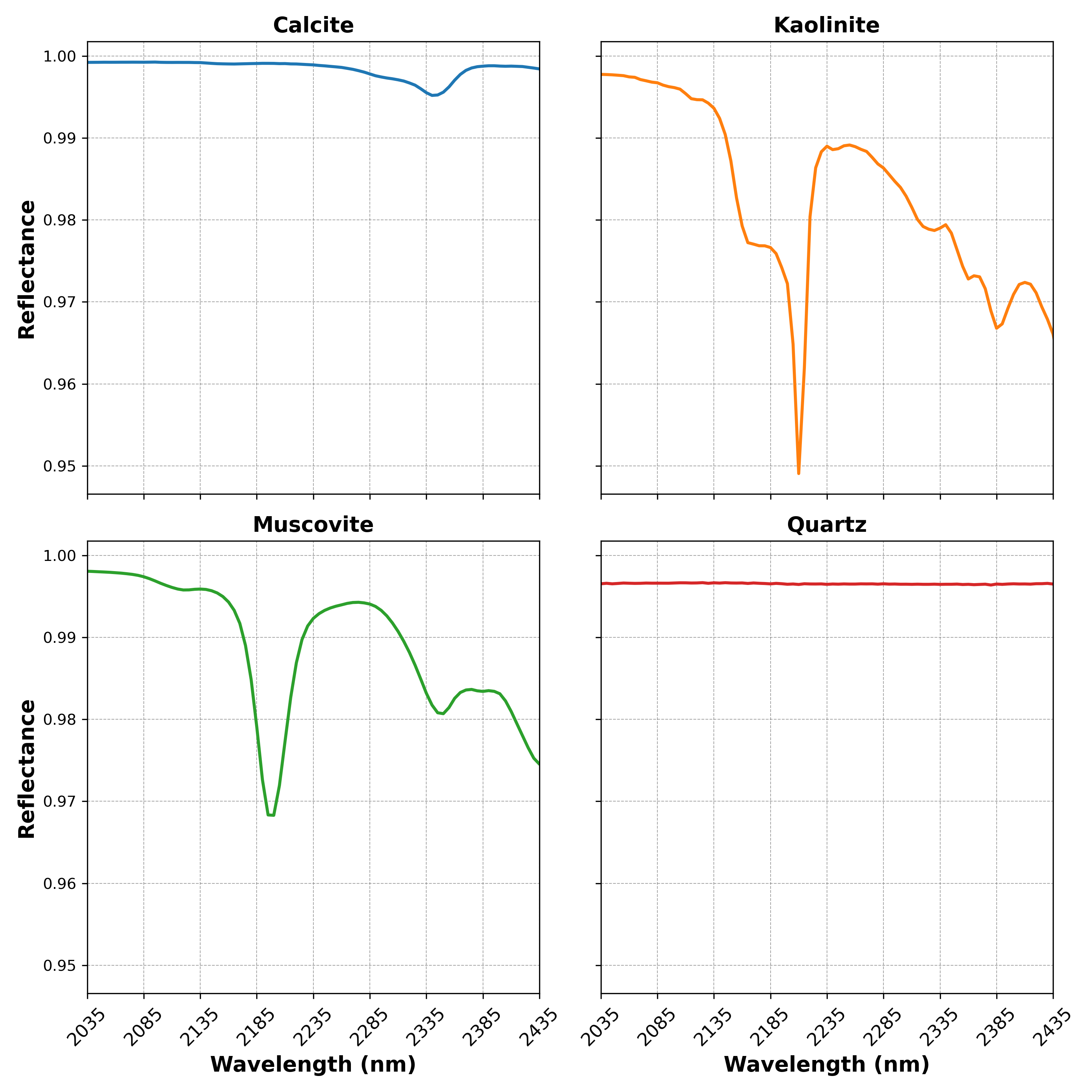
For the first test, suppose we have four mineral endmembers (example taken from USGS Spectral Library), as shown below.

We’ll generate 1000 synthetic mixtures with the following conditions:

1. The mixtures follow the linear mixture model equation.
2. Noise is normally distributed with a mean of \(0\) and a standard deviation chosen randomly between \(10^{-5}\) and \(10^{-3}\).

The accuracy of the spectral unmixing using the three distance metrics are shown below:

In this case, Euclidean distance clearly outperforms the other two metrics, as it is well-suited for data with normally distributed noise. Under these conditions, minimizing Euclidean distance is equivalent to maximum likelihood estimation.

Test 02: Mixture with Random ‘Spikes’

For the second test, instead of adding normal noise, this time we add random “spikes,” where each wavelength band has a \(1\%\) chance of being randomly increased or decreased by a value between \(0.05\) and \(0.2\). While this type of noise is not common in remote sensing or spectroscopy, it will help us illustrate the strengths of Manhattan distance. The accuracy of the spectral unmixing of these synthetic mixtures are shown below:

Here, Manhattan distance outperforms the other metrics. Manhattan distance is known to be more robust to extreme outliers than Euclidean distance, which squares the error term, making it sensitive to outliers. In contrast, Manhattan distance only takes the absolute value of location differences, making it less affected by outliers.

Test 03: Mixture with Brightness Difference

While random spikes in reflectance values may not be common in spectroscopy or remote sensing, brightness differences and inaccurate endmembers spectra are issues that often arise with real datasets. To illustrate this problem, let’s randomly add random constant between \(-0.2\) to \(0.2\) to the mixture. This experiment is a simplified simulation of real world scenario where different terrains and illumination condition might cause the sensor to recieve the signal with different intensity if not corrected appropriately.

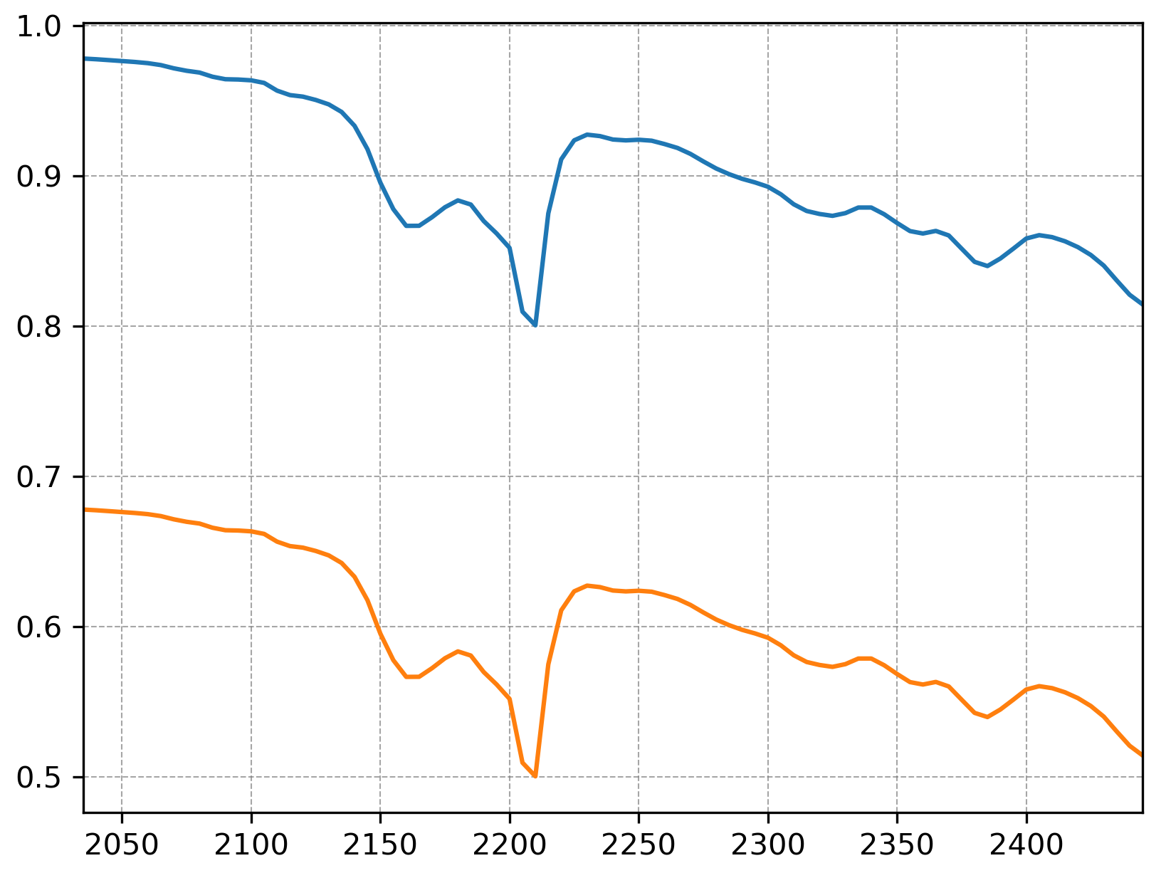
In this case, angular distance (or SAM) has the lowest error, as it essentially ignores magnitude (brightness) differences and focuses on the shape of the spectra. To illustrate further, take a look at the two spectra below:

The two spectra above have identical shape but different brightness values. These two spectra may be considered different by Manhattan and Euclidean distances, but angular distance would see them as identical. This feature is one reason why angular distance is widely used in remote sensing applications, where brightness differences due to terrains and illuminations effects are common.

Test 04: A More Complicated Mixture

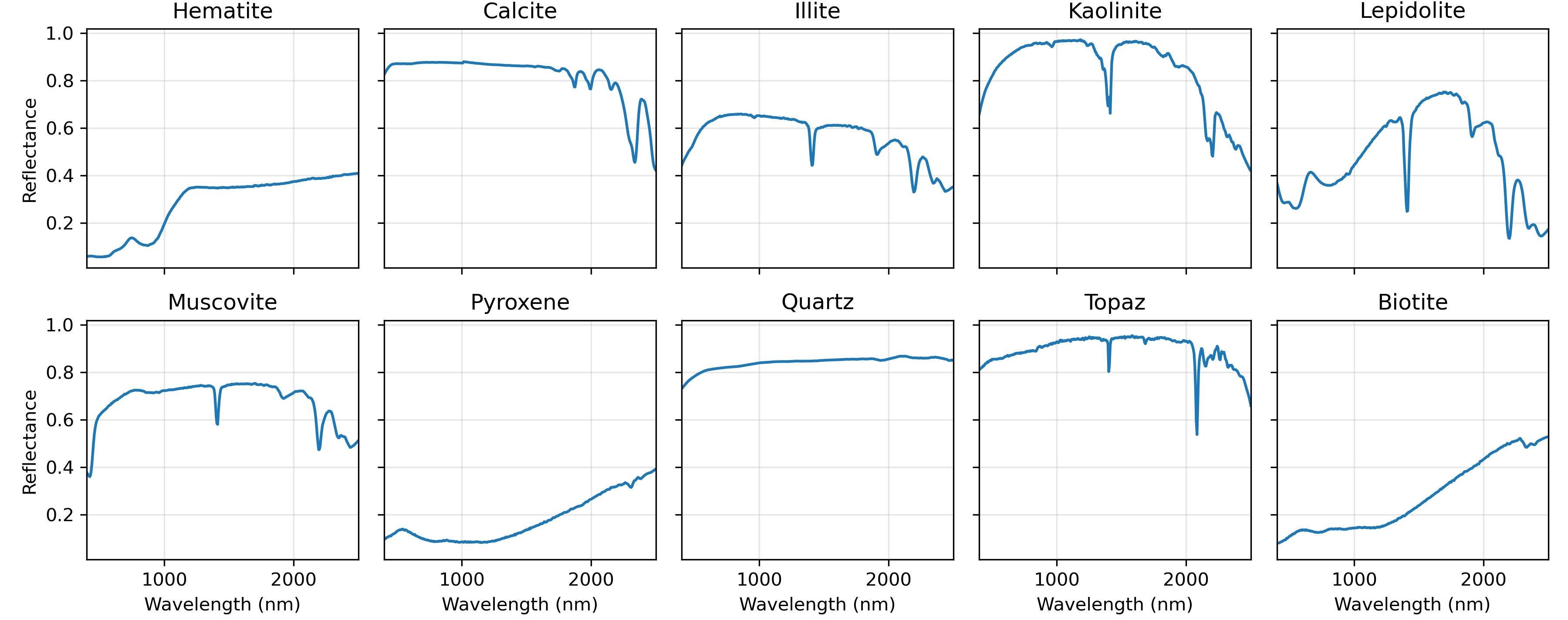
Now let’s consider a more complex scenario. We will use a larger spectral library, selecting 10 minerals from the USGS spectral library. To generate a mixture, we will randomly select between 2 to 4 endmembers from this library. Since the actual selected minerals are unknown, all 10 possible endmembers will be included in the unmixing process. This situation, where many variables (10 possible endmembers) are considered, but only a few (2–4 endmembers) are non-zero, is known as a sparsity problem.

Typically, sparsity issues are addressed by incorporating regularization terms into the optimization function. However, for this simple trial, we will not include any regularization and will apply the same spectral unmixing method used in the previous three tests. This allows us to focus solely on the challenges posed by increased complexity in the spectral library.

We will also add an gaussian noise, uniform noise, gamma noise, poisson noise, and random constant as brightness modifier. The image below ilustrate each of the noises:

The unmixing accuracy results are shown in histograms below:

Manhattan distance performed exceptionally well in this last case study, which probably can be attributed to its robustness to ouliers and more varying noise types. Despite this, its non-differentiable nature (since its an absolute value function) makes it less appealing for gradient-based optimization algorithms, especially for larger, more complex datasets. For this particular test, Manhattan distance takes 43 seconds for 1,000 data points, compared to 14 seconds for Euclidean distance and 11 seconds for angular distance.

This study highlights the importance of carefully selecting the appropriate distance metric based on the nature of the data and the problem being addressed. While Euclidean distance is often the default choice, Manhattan distance or angular distance can outperform it in specific scenarios, as demonstrated in the experiments above.

On a final note, it’s important to emphasize that the unmixing approach presented here operates under the assumption of a perfect model and data. In real-world scenarios, this is rarely the case, so we should generally expect the results to be slightly less accurate. However, it’s crucial to acknowledge that spectral unmixing inherently involves significant uncertainty. A more robust approach to address this uncertainty is to adopt a Bayesian framework, which offers a natural way to model such problems. This will be the topic of our next discussion.