Bayesian Spectral Unmixing

In the previous post we discussed how spectral unmixing inherently suffers from uncertainty—stemming both from the data and the model. Traditional optimization approaches, like the one we used earlier, often assume that these uncertainties are either negligible or nonexistent. However, in practice, this is rarely the case.

In this post, we’ll take a brief look at the Bayesian approach to spectral unmixing, which explicitly accounts for these uncertainties. By incorporating them into the model, we propagate the uncertainty through to the final results. Instead of a single vector of mineral abundances, the Bayesian approach provides a probability distribution for these abundances, offering deeper insight into the confidence we have in our estimates.

While we won’t dive too deeply into the math, a basic formulation helps set the stage. The linear mixture model can be expressed as:

\[\mathbf{y} = \mathbf{E} \mathbf{a} + \mathbf{e}\]

where:

• \(\mathbf{y}\) is the observed spectrum,
• \(\mathbf{E}\) is the endmembers matrix,
• \(\mathbf{a}\) is the abundance vector,
• \(\mathbf{e}\) represents error terms/uncertainty.

Context for this post: We are focusing on unmixing for minerals on particulate surfaces (e.g., rock surfaces). Due to multiple-scattering effects, the linear relationship above does not hold when using reflectance data. Instead, we will use the Single Scattering Albedo (SSA) which derived from Hapke’s Model, as it better handles these effect. For those interested in the underlying theory, I highly recommend consulting this book; these two papers that really helps me a lot with the subject: [1], [2]; or other sources (including my thesis😉)

Bayesian Framework

Following Bayes’ Theorem, we can represent the spectral unmixing problem as:

\[P(\mathbf{a}, \sigma^2 \mid \mathbf{y}, \mathbf{E}) \propto P(\mathbf{y} \mid \mathbf{a}, \sigma^2, \mathbf{E}) P(\mathbf{a}) P(\sigma^2)\]

where:

• \(P(\mathbf{a}, \sigma^2 \mid \mathbf{y}, \mathbf{E})\) is the posterior distribution of the abundance vector and error variance given the observed spectrum and endmembers,
• \(P(\mathbf{y} \mid \mathbf{a}, \sigma^2, \mathbf{E})\) is the likelihood of the observed spectrum,
• \(P(\mathbf{a})\) is the prior distribution of the abundance vector,
• \(P(\sigma^2)\) is the prior distribution of the error variance,
• and \(\propto\) denote proportionality

We assume that the error term \(\mathbf{e}\) is normally distributed, giving us a Normal likelihood:

\[P(\mathbf{y} \mid \mathbf{a}, \sigma^2, \mathbf{E}) = \mathcal{N}(\mathbf{y} \mid \mathbf{E}\mathbf{a}, \sigma^2\mathbf{I}),\]

where \(\mathbf{I}\) is the identity matrix.

For the abundance vector \(\mathbf{a}\), we use a Dirichlet prior to enforce the non-negativity and sum-to-one constraints:

\[P(\mathbf{a}) = \mathcal{D}(\mathbf{a} \mid \boldsymbol{\alpha}),\]

where \(\boldsymbol{\alpha}\) is the concentration parameter.

For the error variance \(\sigma^2\), we assign a Half-Cauchy prior:

\[P(\sigma^2) = \mathcal{HC}(\sigma^2 \mid \beta),\]

with the scale hyperparamter \(\beta\) given a Unifrom prior such as:

\[P(\beta) = \mathcal{U}(\beta \mid 0, 0^{-4}).\]

Therefore, we can summarize the hierarchical structure of the random variables as:

\[\mathbf{y} \sim \mathcal{N}(\mathbf{E}\mathbf{a}, \sigma^2\mathbf{I})\] \[\mathbf{a} \sim \mathcal{D}(\boldsymbol{\alpha})\] \[\sigma^2 \sim \mathcal{HC}(\beta)\] \[\beta \sim \mathcal{U}(0, 10^{-4})\]

As you might guess, this formulation of the posterior distribution cannot be solved analytically. Instead, we use Markov Chain Monte Caelo (MCMC) to sample and estimate the posterior. For educational purposes, I’ve implemented a custom sampler based on the Metropolis-Hastings Random Walk in Python. In practice, however, modern samplers like NUTS (No-U-Turn Sampler) in an established library such as PyMC are often preferable. They offer a more efficient and streamlined sampling process, sparing users the burden of directly managing the nasty mathematics behind these algorithms.

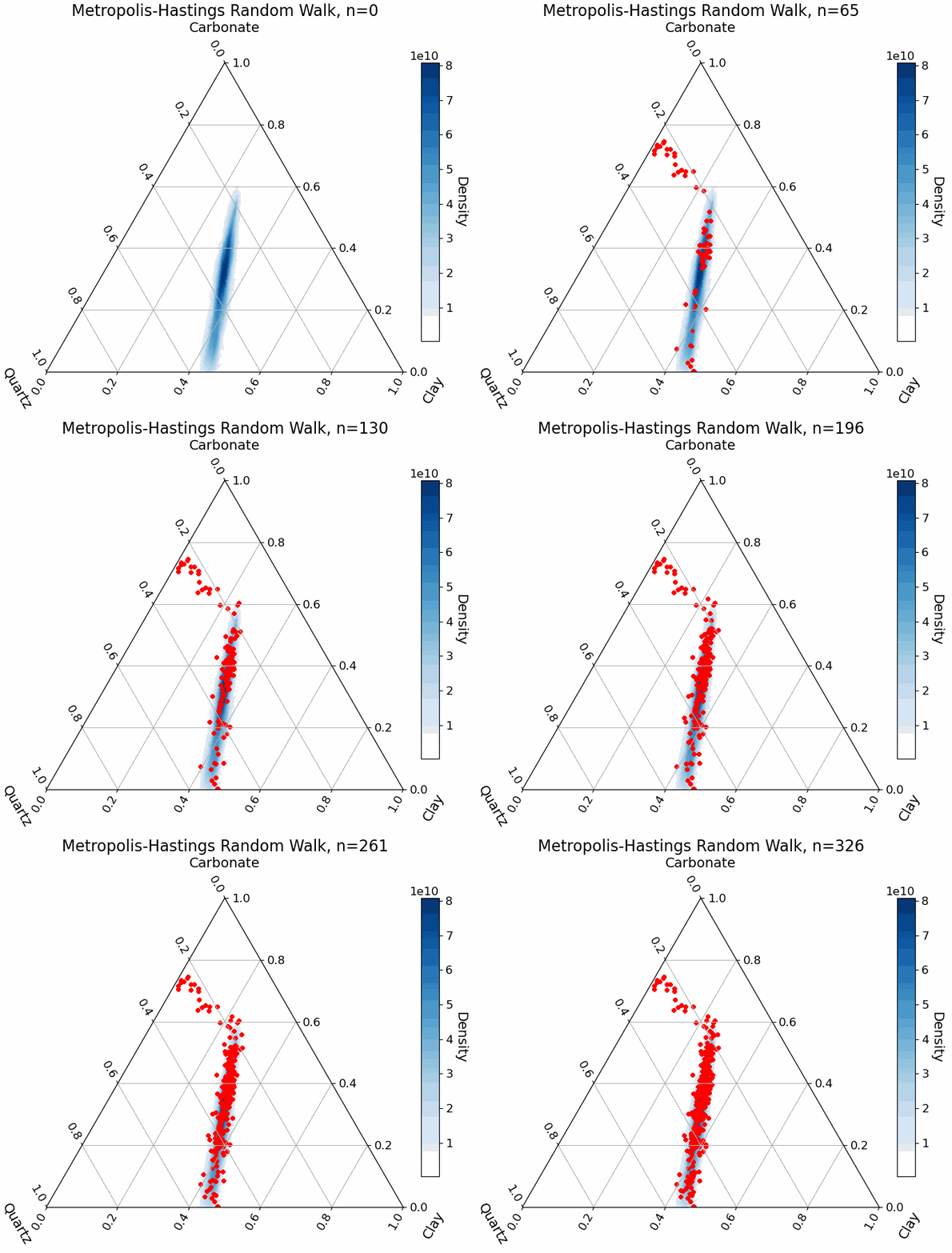
In the Metropolis-Hastings algorithm, we iteratively draw samples from the posterior. For each new sample, we evaluate its probability relative to the previous sample. The sample is either accepted or rejected based on this evaluation. Over many iterations, the density of accepted samples approximates the true posterior distribution.

For illustration, the animation below shows the random walk process for sampling abundance parameters in a mixture of three endmembers. The blue regions represent the true target distribution. Notice how the sampler, starting from a random point in the parameter space, gradually converges to the high-probability regions:

Practical Example

In this example, we will analyze a sandstone rock sample. Rock samples are ideal for testing this method since they represent natural surfaces and still allow us to conduct other detailed analytical measurements with laboratory instruments to produce high-quality ‘ground truth’ data for comparison with our results.

For the endmembers, we consider three primary components of sandstone: quartz (grains), clay (matrix), and carbonates (cement). The endmember spectra for these minerals are assumed to be known, either from direct laboratory measurements, spectral libraries, or endmember extraction algorithms for hyperspectral imagery. We begin with a single mixed spectrum, as shown in the image below:

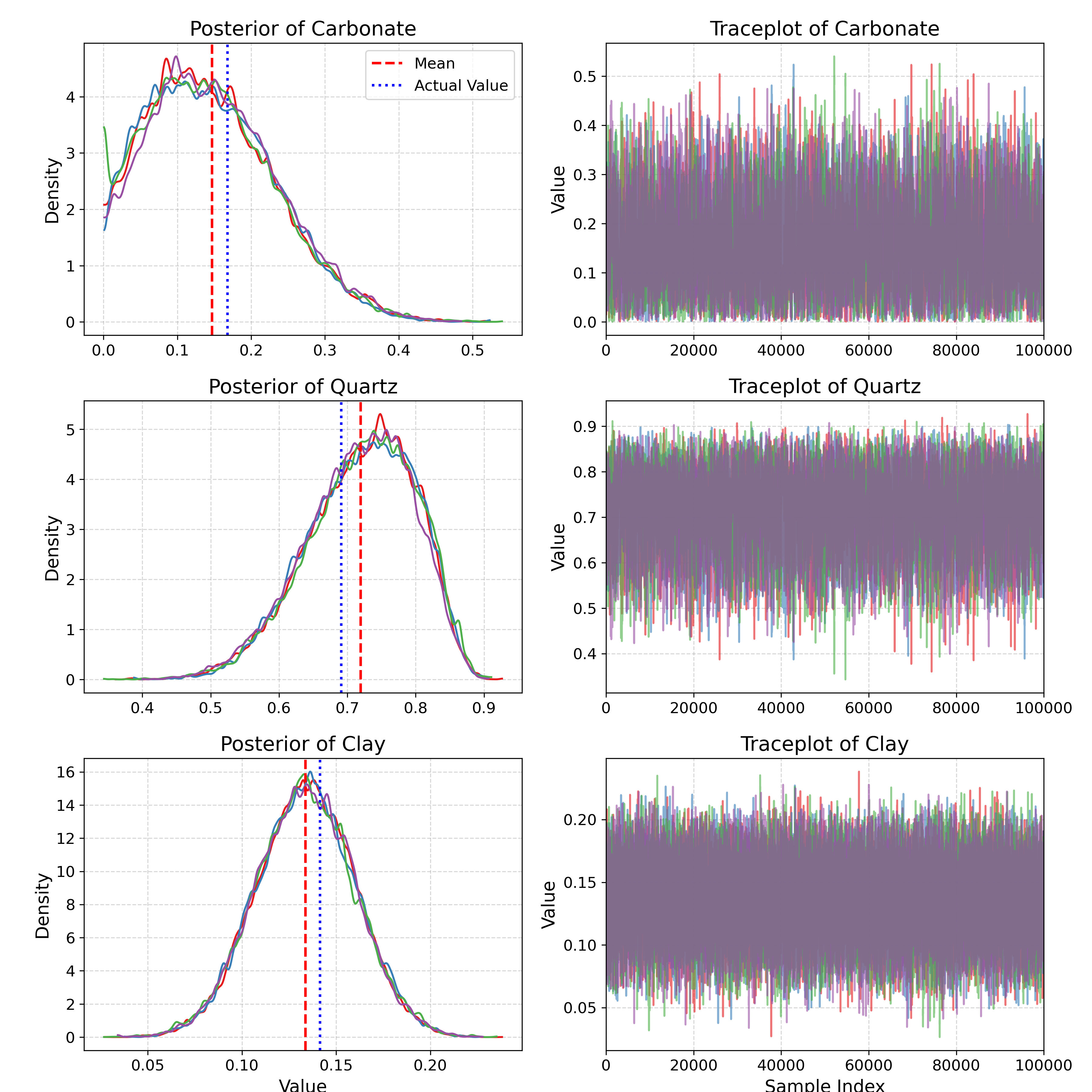
Using our Metropolis-Hastings sampler, we draw four chains of \(10^5\) random samples, tuning them carefully to ensure we only consider representative samples. For simplicity, we focus solely on the mineral abundances and omit other parameters. Below, we display the abundance trace plots alongside their corresponding marginal posterior distributions. The mean value (expected values) of the samples and the true abundance values are also shown as comparison. The RMSE for this result is 0.0209.

There are some cool things that we can do with the posteriors. For instance, we can visualize parameter correlations using a corner plot, as shown below. Note as well how we denote the result with some notation such as: \(0.14_{-0.12}^{+0.16}\) where the central value represents the expected value, while the subscript and superscript indicate the range of possible value within 90% confidence interval.

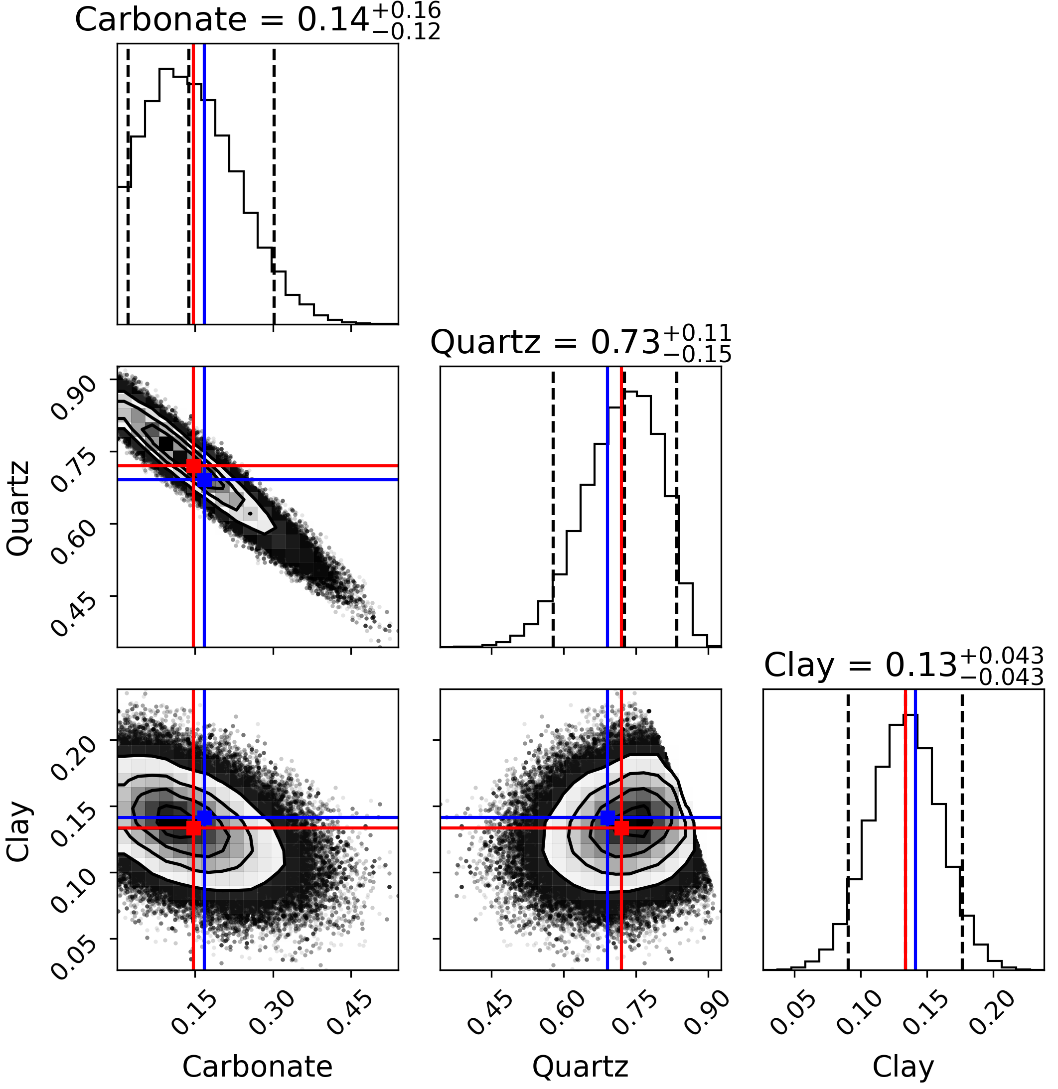
Corner plots are a really useful visualization, especially for high-dimensional parameter spaces. For this three-parameter example, however, we can also visualize the posterior on a ternary diagram:

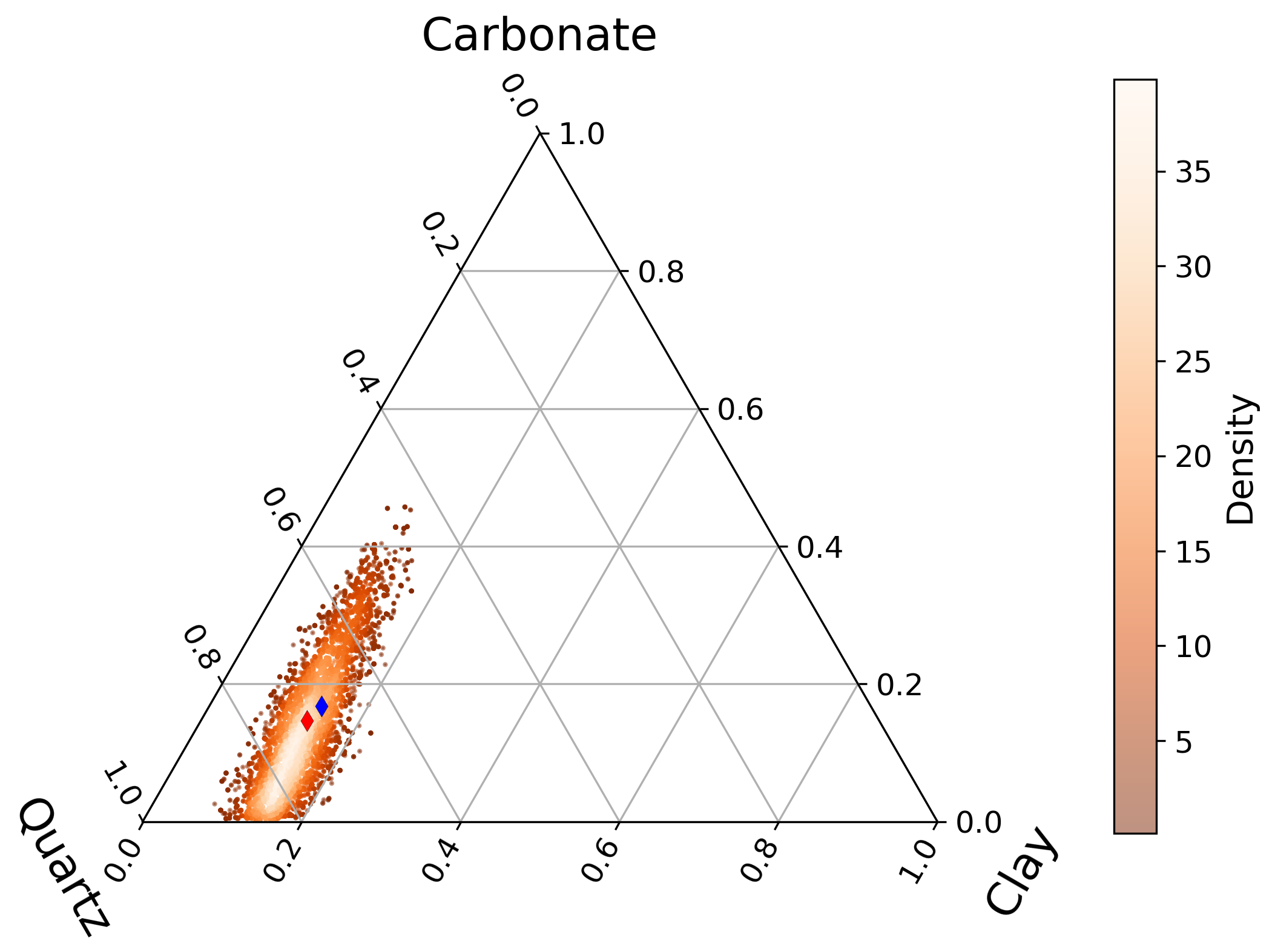
The corner and ternary plots reveal a strong correlation between carbonate and quartz abundances. As carbonate increases, the algorithm compensates by reducing quartz to maintain a reasonable modeled spectrum that aligns with the observed data. Instead of a single modeled spectrum, the output is a distribution of spectra, visualized below:

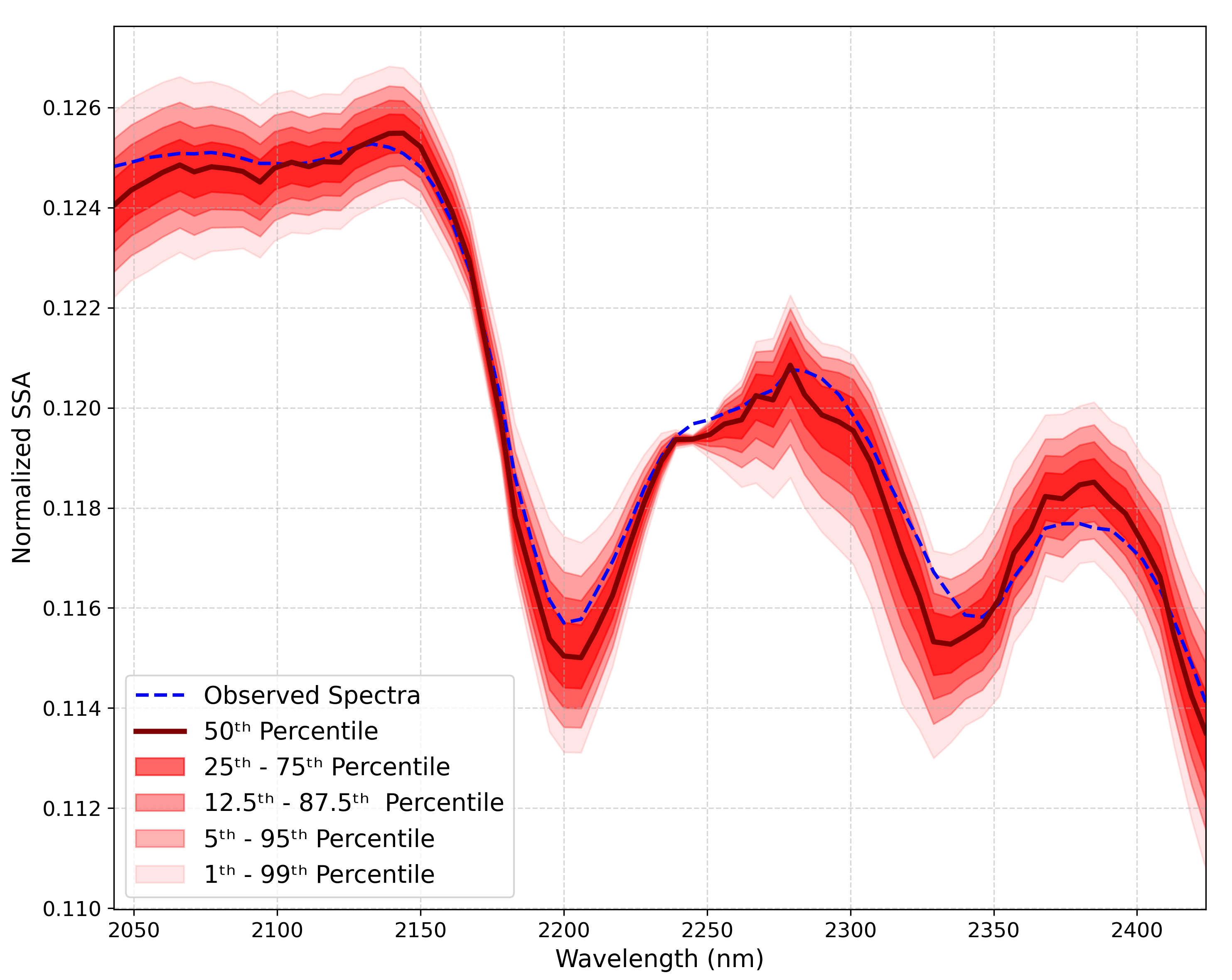
This visualization highlights that, given the data and assumed uncertainties, the reasonable set of modeled spectra is represented by the 2D Normal distribution visualize by its percentiles as shown on the image above.

Hyperspectral Images

The same process applies to hyperspectral images on a pixel-by-pixel basis. Here, we analyze a hyperspectral image of a sandstone drill core sample. Remember that for individual spectra (or also pixel in this case) the sampler will need to take and store \(10^{5}\) sample for each parameters. This means that the final result will be a huge 4D array, and the computation might take some time, depending on the efficiency of the sampling algorithm used. Below, we visualize the expected abundance values for each endmember and their 90% confidence intervals range:

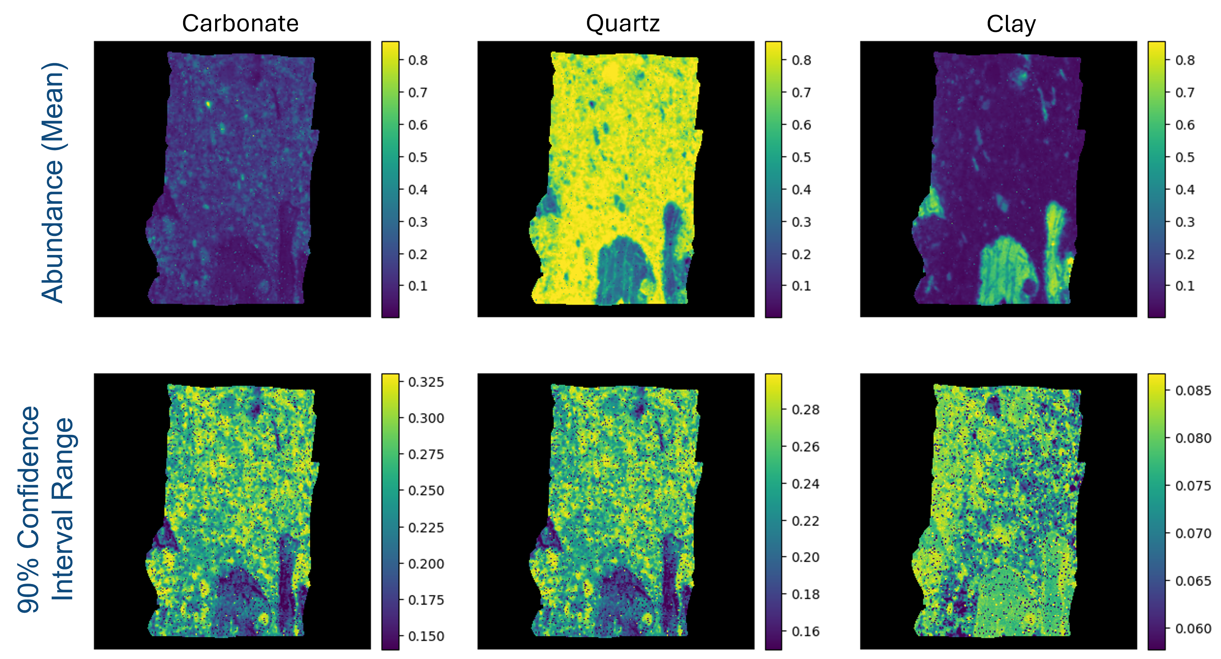
Comparing our bulk results with QEMSCAN results, we can achieve excellent agreement with an RMSE of 0.0186.

It’s important to highlight that quantification through imaging techniques like this does more than just identify mineral abundances—it also provides a detailed view of the rock’s texture. By analyzing mineral distributions and their spatial relationships, we can potentially infer other critical physical properties of the rock such as porosity and permeability, which might be really usefult for application like reservoir characterization and groundwater studies.

The inclusion of uncertainty measurement in spectral unmixing offers an important insights into the reliability of the results. Rather than relying solely on point estimates, we gain a more nuanced understanding of the possible variations and correlations in parameter space. This is particularly valuable when making decisions based on complex data, as it helps avoid overconfidence and identifies parameters requiring further refinement. In mineral quantification, understanding uncertainties can reveal how robust the mineral abundance estimates are, guiding both data interpretation and future analyses.

Hyperspectral imaging, as demonstrated in this example, have the potential for a more fast and cost-effective alternative of mineral abundance mapping compared to other laboratory method. Moreover, it has the potential to scale up to airborne and satellite platforms, making it one of a kind method for larger-scale mineral mapping and monitoring.